Swift Tutorial for RCC Midway Cluster

This tutorial is viewable at: http://swiftlang.org/tutorials/midway/tutorial.html

Introduction: Why Parallel Scripting?

Swift is a simple scripting language for executing many instances of ordinary application programs on distributed parallel resources. Swift scripts run many copies of ordinary programs concurrently, using statements like this:

foreach protein in proteinList {
  runBLAST(protein);
}

Swift acts like a structured "shell" language. It runs programs concurrently as soon as their inputs are available, reducing the need for complex parallel programming. Swift expresses your workflow in a portable fashion: The same script runs on multicore computers, clusters, clouds, grids, and supercomputers.

In this tutorial, you’ll be able to first try a few Swift examples (parts 1-3) on a Midway login host, to get a sense of the language. Then in parts 4-6 you’ll run similar workflows on Midway compute nodes, and see how more complex workflows can be expressed with Swift scripts.

Swift tutorial setup

If you are using a temporary/guest account to access Midway, follow the instructions at http://docs.rcc.uchicago.edu/tutorials/intro-to-rcc-workshop.html for more information on using a yubikey to log in.

Once you are logged into the Midway login host, run the following commands to set up your environment.

$ cd $HOME
$ wget http://swiftlang.org/tutorials/midway/swift-midway-tutorial.tar.gz
$ tar xvfz swift-midway-tutorial.tar.gz
$ cd swift-midway-tutorial
$ source setup.sh

Verify your environment

To verify that Swift loaded, do:

$ swift -version  # verify that you have Swift 0.95 RC1

If you re-login or open new ssh sessions, you must re-run source setup.sh in each ssh shell/window.

To check out the tutorial scripts from SVN

If you later want to get the most recent version of this tutorial from the Swift Subversion repository, do:

$ svn co https://svn.ci.uchicago.edu/svn/vdl2/SwiftTutorials/swift-midway-tutorial

This will create a directory called "swift-midway-tutorial" which contains all of the files used in this tutorial.

Simple "science applications" for the workflow tutorial

This tutorial is based on two intentionally trivial example programs, simulation and stats, (implemented as bash shell scripts) that serve as easy-to-understand proxies for real science applications. These "programs" behave as follows.

simulate.sh

The simulation script serves as a trivial proxy for any more complex scientific simulation application. It generates and prints a set of one or more random integers in the range [0-2^62) as controlled by its command line arguments, which are:

$ simulate -help
simulate: usage:
    -b|--bias       offset bias: add this integer to all results
    -B|--biasfile   file of integer biases to add to results
    -l|--log        generate a log in stderr if not null
    -n|--nvalues    print this many values per simulation
    -r|--range      range (limit) of generated results
    -s|--seed       use this integer [0..32767] as a seed
    -S|--seedfile   use this file (containing integer seeds [0..32767]) one per line
    -t|--timesteps  number of simulated "timesteps" in seconds (determines runtime)
    -x|--scale      scale the results by this integer
    -h|-?|?|--help  print this help

All of these arguments are optional, with default values indicated above as [n].

With no arguments, simulate prints 1 number in the range of 1-100. Otherwise it generates n numbers of the form (R*scale)+bias where R is a random integer. By default it logs information about its execution environment to stderr. Here’s some examples of its usage:

$ simulate 2>log
      51
$ head -5 log

Called as: /home/davidkelly999/swift-midway-tutorial/app/simulate:
Start time: Mon Dec  2 13:47:41 CST 2013
Running as user: uid=88848(davidkelly999) gid=88848(davidkelly999) groups=88848(davidkelly999),10008(rcc),10030(pi-gavoth),10031(sp-swift),10036(swift),10058(pi-joshuaelliott),10084(pi-wilde),10118(cron-account),10124(cmts),10138(cmtsworkshop)

$ simulate -n 4 -r 1000000 2>log
  239454
  386702
   13849
  873526

$ simulate -n 3 -r 1000000 -x 100 2>log
 6643700
62182300
 5230600

$ simulate -n 2 -r 1000 -x 1000 2>log
  565000
  636000

$ time simulate -n 2 -r 1000 -x 1000 -t 3 2>log
  336000
  320000
real    0m3.012s
user    0m0.005s
sys     0m0.006s

stats

The stats script serves as a trivial model of an "analysis" program. It reads N files each containing M integers and simply prints the average of all those numbers to stdout. Similarly to simulate it logs environmental information to the stderr.

$ ls f*
f1  f2  f3  f4

$ cat f*
25
60
40
75

$ stats f* 2>log
50

Basic of the Swift language with local execution

A Summary of Swift in a nutshell

Swift scripts are text files ending in .swift The swift command runs on any host, and executes these scripts. swift is a Java application, which you can install almost anywhere. On Linux, just unpack the distribution tar file and add its bin/ directory to your PATH.
Swift scripts run ordinary applications, just like shell scripts do. Swift makes it easy to run these applications on parallel and remote computers (from laptops to supercomputers). If you can ssh to the system, Swift can likely run applications there.
The details of where to run applications and how to get files back and forth are described in configuration files separate from your program. Swift speaks ssh, PBS, Condor, SLURM, LSF, SGE, Cobalt, and Globus to run applications, and scp, http, ftp, and GridFTP to move data.
The Swift language has 5 main data types: boolean, int, string, float, and file. Collections of these are dynamic, sparse arrays of arbitrary dimension and structures of scalars and/or arrays defined by the type declaration.
Swift file variables are "mapped" to external files. Swift sends files to and from remote systems for you automatically.
Swift variables are "single assignment": once you set them you can’t change them (in a given block of code). This makes Swift a natural, "parallel data flow" language. This programming model keeps your workflow scripts simple and easy to write and understand.
Swift lets you define functions to "wrap" application programs, and to cleanly structure more complex scripts. Swift app functions take files and parameters as inputs and return files as outputs.
A compact set of built-in functions for string and file manipulation, type conversions, high level IO, etc. is provided. Swift’s equivalent of printf() is tracef(), with limited and slightly different format codes.
Swift’s foreach {} statement is the main parallel workhorse of the language, and executes all iterations of the loop concurrently. The actual number of parallel tasks executed is based on available resources and settable "throttles".
In fact, Swift conceptually executes all the statements, expressions and function calls in your program in parallel, based on data flow. These are similarly throttled based on available resources and settings.
Swift also has if and switch statements for conditional execution. These are seldom needed in simple workflows but they enable very dynamic workflow patterns to be specified.

We’ll see many of these points in action in the examples below. Lets get started!

Part 1: Run a single application under Swift

The first swift script, p1.swift, runs simulate to generate a single random number. It writes the number to a file.

p1.swift

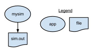
type file;

app (file o) simulation ()
{
  simulate stdout=filename(o);
}

file f <"sim.out">;
f = simulation();

To run this script, run the following command:

$ cd part01
$ swift p1.swift
Swift 0.94.1 RC2 swift-r6895 cog-r3765

RunID: 20130827-1413-oa6fdib2
Progress:  time: Tue, 27 Aug 2013 14:13:33 -0500
Final status: Tue, 27 Aug 2013 14:13:33 -0500  Finished successfully:1
$ cat sim.out
      84
$ swift p1.swift
$ cat sim.out
      36

To cleanup the directory and remove all outputs (including the log files and directories that Swift generates), run the cleanup script which is located in the tutorial PATH:

$ cleanup

You’ll also find a Swift configuration file in each partNN directory of this tutorial. This file specifies the environment-specific details of how to run. These files will be explained in more detail in parts 4-6, and can be ignored for now.

Part 2: Running an ensemble of many apps in parallel with a "foreach" loop

The p2.swift script introduces the foreach parallel iteration construct to run many concurrent simulations.

p2.swift

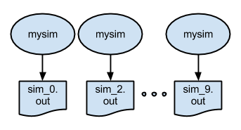
type file;

app (file o) simulation ()
{
  simulate stdout=filename(o);
}

foreach i in [0:9] {
  file f <single_file_mapper; file=strcat("output/sim_",i,".out")>;
  f = simulation();
}

The script also shows an example of naming the output files of an ensemble run. In this case, the output files will be named output/sim_N.out.

To run the script and view the output:

$ cd ../part02
$ swift p2.swift
$ ls output
sim_0.out  sim_1.out  sim_2.out  sim_3.out  sim_4.out  sim_5.out  sim_6.out  sim_7.out  sim_8.out  sim_9.out
$ more output/*
::::::::::::::
output/sim_0.out
::::::::::::::
      44
::::::::::::::
output/sim_1.out
::::::::::::::
      55
...
::::::::::::::
output/sim_9.out
::::::::::::::
      82

Part 3: Analyzing results of a parallel ensemble

After all the parallel simulations in an ensemble run have completed, its typically necessary to gather and analyze their results with some kind of post-processing analysis program or script. p3.swift introduces such a postprocessing step. In this case, the files created by all of the parallel runs of simulation will be averaged by by the trivial "analysis application" stats:

p3.swift

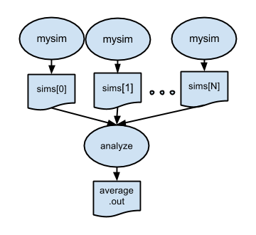
type file;

app (file o) simulation (int sim_steps, int sim_range, int sim_values)
{
  simulate "--timesteps" sim_steps "--range" sim_range "--nvalues" sim_values stdout=filename(o);
}

app (file o) analyze (file s[])
{
  stats filenames(s) stdout=filename(o);
}

int nsim   = toInt(arg("nsim","10"));
int steps  = toInt(arg("steps","1"));
int range  = toInt(arg("range","100"));
int values = toInt(arg("values","5"));

file sims[];

foreach i in [0:nsim-1] {
  file simout <single_file_mapper; file=strcat("output/sim_",i,".out")>;
  simout = simulation(steps,range,values);
  sims[i] = simout;
}

file stats<"output/average.out">;
stats = analyze(sims);

To run:

$ cd part03
$ swift p3.swift

Note that in p3.swift we expose more of the capabilities of the simulate application to the simulation() app function:

app (file o) simulation (int sim_steps, int sim_range, int sim_values)
{
  simulate "--timesteps" sim_steps "--range" sim_range "--nvalues" sim_values stdout=@filename(o);
}

p3.swift also shows how to fetch application-specific values from the swift command line in a Swift script using arg() which accepts a keyword-style argument and its default value:

int nsim   = toInt(arg("nsim","10"));
int steps  = toInt(arg("steps","1"));
int range  = toInt(arg("range","100"));
int values = toInt(arg("values","5"));

Now we can specify that more runs should be performed and that each should run for more timesteps, and produce more that one value each, within a specified range, using command line arguments placed after the Swift script name in the form -parameterName=value:

$ swift p3.swift -nsim=3 -steps=10 -values=4 -range=1000000

Swift 0.94.1 RC2 swift-r6895 cog-r3765

RunID: 20130827-1439-s3vvo809
Progress:  time: Tue, 27 Aug 2013 14:39:42 -0500
Progress:  time: Tue, 27 Aug 2013 14:39:53 -0500  Active:2  Stage out:1
Final status: Tue, 27 Aug 2013 14:39:53 -0500  Finished successfully:4

$ ls output/
average.out  sim_0.out  sim_1.out  sim_2.out
$ more output/*
::::::::::::::
output/average.out
::::::::::::::
651368
::::::::::::::
output/sim_0.out
::::::::::::::
  735700
  886206
  997391
  982970
::::::::::::::
output/sim_1.out
::::::::::::::
  260071
  264195
  869198
  933537
::::::::::::::
output/sim_2.out
::::::::::::::
  201806
  213540
  527576
  944233

Now try running (-nsim=) 100 simulations of (-steps=) 1 second each:

$ swift p3.swift -nsim=100 -steps=1
Swift 0.94.1 RC2 swift-r6895 cog-r3765

RunID: 20130827-1444-rq809ts6
Progress:  time: Tue, 27 Aug 2013 14:44:55 -0500
Progress:  time: Tue, 27 Aug 2013 14:44:56 -0500  Selecting site:79  Active:20  Stage out:1
Progress:  time: Tue, 27 Aug 2013 14:44:58 -0500  Selecting site:58  Active:20  Stage out:1  Finished successfully:21
Progress:  time: Tue, 27 Aug 2013 14:44:59 -0500  Selecting site:37  Active:20  Stage out:1  Finished successfully:42
Progress:  time: Tue, 27 Aug 2013 14:45:00 -0500  Selecting site:16  Active:20  Stage out:1  Finished successfully:63
Progress:  time: Tue, 27 Aug 2013 14:45:02 -0500  Active:15  Stage out:1  Finished successfully:84
Progress:  time: Tue, 27 Aug 2013 14:45:03 -0500  Finished successfully:101
Final status: Tue, 27 Aug 2013 14:45:03 -0500  Finished successfully:101

We can see from Swift’s "progress" status that the tutorial’s default parameters for local execution allow Swift to run up to 20 application invocations concurrently on the login node. We’ll look at this in more detail in the next sections where we execute applications on the site’s compute nodes.

Running applications on Midway compute nodes with Swift

Part 4: Running a parallel ensemble on Midway compute nodes

p4.swift will run our mock "simulation" applications on Midway compute nodes. The script is similar to as p3.swift, but specifies that each simulation app invocation should additionally return the log file which the application writes to stderr.

Now when you run swift p4.swift you’ll see that two types output files will placed in the output/ directory: sim_N.out and sim_N.log. The log files provide data on the runtime environment of each app invocation. For example:

$ cat output/sim_0.log
Called as: /home/davidkelly999/swift-midway-tutorial/app/simulate: --timesteps 1 --range 100 --nvalues 5

Start time: Mon Dec  2 12:17:06 CST 2013
Running as user: uid=88848(davidkelly999) gid=88848(davidkelly999) groups=88848(davidkelly999),10008(rcc),10030(pi-gavoth),10031(sp-swift),10036(swift),10058(pi-joshuaelliott),10084(pi-wilde),10118(cron-account),10124(cmts),10138(cmtsworkshop)
Running on node: midway002
Node IP address: 10.50.181.2 172.25.181.2

Simulation parameters:

bias=0
biasfile=none
initseed=none
log=yes
paramfile=none
range=100
scale=1
seedfile=none
timesteps=1
output width=8

Environment:

ANTLR_ROOT=/software/antlr-2.7-el6-x86_64
ANT_HOME=/software/ant-1.8.4-all
ANT_HOME_modshare=/software/ant-1.8.4-all:3
...

Swift’s swift.properties configuration file allows many parameters to specify how jobs should be run on a given cluster.

Consider for example that Midway has several Slurm partitions. The sandyb partition has 16 cores, and the westmere partition has 12 cores. Depending on the application and which partitions are busy, you may want to modify where you run.

Here is an example of the swift.properties in the part04 directory:

site=westmere
site.westmere.slurm.reservation=workshop
site.westmere.slurm.exclusive=false

The first line, site=westmere, allows you to define which partition to run on. Swift includes templates for each partition that provides some reasonable default values. Other valid partitions are amd, bigmem, gpu, local, and sandyb.

The second and third line override some of the default values, by specifying a reservation that will be used for this session, and enabling node sharing.

Try changing the queue to run on the sandyb queue. The new swift.properties should look like this:

site=sandyb
site.sandyb.slurm.reservation=workshop
site.sandyb.slurm.exclusive=false

Performing larger Swift runs

To test with larger runs, there are two changes that are required. The first is a change to the command line arguments. The example below will run 1000 simulations with each simulation taking 5 seconds.

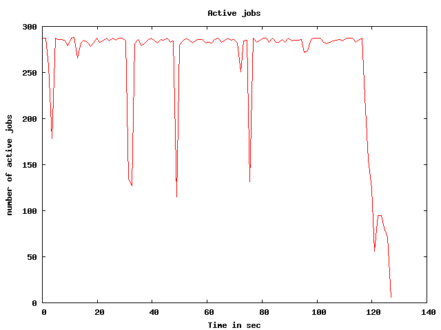
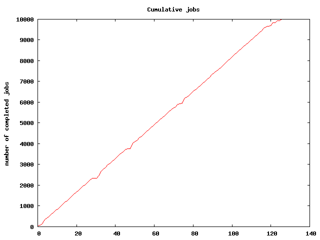
$ swift p6.swift -steps=5 -nsim=1000

Plotting run activity

The tutorial bin directory in your PATH provides a script plot.sh to plot the progress of a Swift script. It generates two image files: activeplot.png, which shows the number of active jobs over time, and cumulativeplot.png, which shows the total number of app calls completed as the Swift script progresses.

After each Swift run, a new run directory is created called runNNN. Each run directory will have a log file with a similar name called runNNN.log. Once you have identified the log file name, run the command plot.sh <logfile>` to generate the plots for that specific run. For example:

$ ls
output  p3.swift  run000  swift.properties

$ cd run000/

$ ls
apps  cf  p3-20131202-2004-0kh4ha6e.d  run000.log  sites.xml

$ plot.sh run000.log

This yields plots like:

Part 5: Controlling the compute-node pools where applications run

This section is under development.

Part 6: Specifying more complex workflow patterns

p6.swift expands the workflow pattern of p4.swift to add additional stages to the workflow. Here, we generate a dynamic seed value that will be used by all of the simulations, and for each simulation, we run an pre-processing application to generate a unique "bias file". This pattern is shown below, followed by the Swift script.

p6.swift

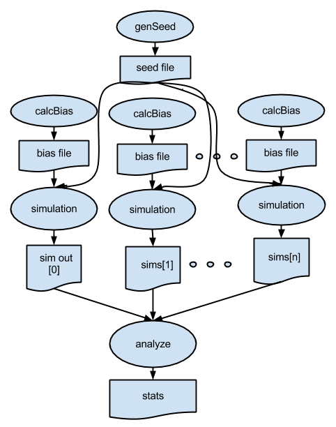
type file;

# app() functions for application programs to be called:

app (file out) genseed (int nseeds)
{
  simulate "-r" 2000000 "-n" nseeds stdout=@out;
}

app (file out) genbias (int bias_range, int nvalues)
{
  simulate "-r" bias_range "-n" nvalues stdout=@out;
}

app (file out, file log) simulation (int timesteps, int sim_range, file bias_file,
                                     int scale, int sim_count, file seed_file)
{
  simulate "-t" timesteps "-r" sim_range "-B" @bias_file "-x" scale
           "-n" sim_count "-S" @seed_file stdout=@out stderr=@log;
}

app (file out, file log) analyze (file s[])
{
  stats filenames(s) stdout=@out stderr=@log;
}

# Command line arguments

int   nsim = toInt(arg("nsim",   "10"));  # number of simulation programs to run
int  steps = toInt(arg("steps",  "1"));   # number of timesteps (seconds) per simulation
int  range = toInt(arg("range",  "100")); # range of the generated random numbers
int values = toInt(arg("values", "10"));  # number of values generated per simulation

# Main script and data
file seedfile <"output/seed.dat">;        # Dynamically generated bias for simulation ensemble

tracef("\n*** Script parameters: nsim=%i range=%i num values=%i\n\n", nsim, range, values);
seedfile = genseed(1);

file sims[];                      # Array of files to hold each simulation output

foreach i in [0:nsim-1] {
  file biasfile <single_file_mapper; file=strcat("output/bias_",i,".dat")>;
  file simout   <single_file_mapper; file=strcat("output/sim_",i,".out")>;
  file simlog   <single_file_mapper; file=strcat("output/sim_",i,".log")>;
  biasfile = genbias(1000, 20);
  (simout,simlog) = simulation(steps, range, biasfile, 1000000, values, seedfile);
  sims[i] = simout;
}

file stats_out<"output/average.out">;
file stats_log<"output/average.log">;
(stats_out,stats_log) = analyze(sims);

Note that the workflow is based on data flow dependencies: each simulation depends on the seed value, calculated in this statement:

seedfile = genseed(1);

and on the bias file, computed and then consumed in these two dependent statements:

  biasfile = genbias(1000, 20);
  (simout,simlog) = simulation(steps, range, biasfile, 1000000, values, seedfile);

To run:

$ cd ../part06
$ swift p6.swift

The default parameters result in the following execution log:

$ swift p6.swift
Swift 0.94.1 RC2 swift-r6895 cog-r3765

RunID: 20130827-1917-jvs4gqm5
Progress:  time: Tue, 27 Aug 2013 19:17:56 -0500

*** Script parameters: nsim=10 range=100 num values=10

Progress:  time: Tue, 27 Aug 2013 19:17:57 -0500  Stage in:1  Submitted:10
Generated seed=382537
Progress:  time: Tue, 27 Aug 2013 19:17:59 -0500  Active:9  Stage out:1  Finished successfully:11
Final status: Tue, 27 Aug 2013 19:18:00 -0500  Finished successfully:22

which produces the following output:

$ ls -lrt output
total 264
-rw-r--r-- 1 p01532 61532     9 Aug 27 19:17 seed.dat
-rw-r--r-- 1 p01532 61532   180 Aug 27 19:17 bias_9.dat
-rw-r--r-- 1 p01532 61532   180 Aug 27 19:17 bias_8.dat
-rw-r--r-- 1 p01532 61532   180 Aug 27 19:17 bias_7.dat
-rw-r--r-- 1 p01532 61532   180 Aug 27 19:17 bias_6.dat
-rw-r--r-- 1 p01532 61532   180 Aug 27 19:17 bias_5.dat
-rw-r--r-- 1 p01532 61532   180 Aug 27 19:17 bias_4.dat
-rw-r--r-- 1 p01532 61532   180 Aug 27 19:17 bias_3.dat
-rw-r--r-- 1 p01532 61532   180 Aug 27 19:17 bias_2.dat
-rw-r--r-- 1 p01532 61532   180 Aug 27 19:17 bias_1.dat
-rw-r--r-- 1 p01532 61532   180 Aug 27 19:17 bias_0.dat
-rw-r--r-- 1 p01532 61532    90 Aug 27 19:17 sim_9.out
-rw-r--r-- 1 p01532 61532 14897 Aug 27 19:17 sim_9.log
-rw-r--r-- 1 p01532 61532 14897 Aug 27 19:17 sim_8.log
-rw-r--r-- 1 p01532 61532    90 Aug 27 19:17 sim_7.out
-rw-r--r-- 1 p01532 61532    90 Aug 27 19:17 sim_6.out
-rw-r--r-- 1 p01532 61532 14897 Aug 27 19:17 sim_6.log
-rw-r--r-- 1 p01532 61532    90 Aug 27 19:17 sim_5.out
-rw-r--r-- 1 p01532 61532 14897 Aug 27 19:17 sim_5.log
-rw-r--r-- 1 p01532 61532    90 Aug 27 19:17 sim_4.out
-rw-r--r-- 1 p01532 61532 14897 Aug 27 19:17 sim_4.log
-rw-r--r-- 1 p01532 61532 14897 Aug 27 19:17 sim_1.log
-rw-r--r-- 1 p01532 61532    90 Aug 27 19:18 sim_8.out
-rw-r--r-- 1 p01532 61532 14897 Aug 27 19:18 sim_7.log
-rw-r--r-- 1 p01532 61532    90 Aug 27 19:18 sim_3.out
-rw-r--r-- 1 p01532 61532 14897 Aug 27 19:18 sim_3.log
-rw-r--r-- 1 p01532 61532    90 Aug 27 19:18 sim_2.out
-rw-r--r-- 1 p01532 61532 14898 Aug 27 19:18 sim_2.log
-rw-r--r-- 1 p01532 61532    90 Aug 27 19:18 sim_1.out
-rw-r--r-- 1 p01532 61532    90 Aug 27 19:18 sim_0.out
-rw-r--r-- 1 p01532 61532 14897 Aug 27 19:18 sim_0.log
-rw-r--r-- 1 p01532 61532     9 Aug 27 19:18 average.out
-rw-r--r-- 1 p01532 61532 14675 Aug 27 19:18 average.log

Each sim_N.out file is the sum of its bias file plus newly "simulated" random output scaled by 1,000,000:

$ cat output/bias_0.dat
     302
     489
      81
     582
     664
     290
     839
     258
     506
     310
     293
     508
      88
     261
     453
     187
      26
     198
     402
     555

$ cat output/sim_0.out
64000302
38000489
32000081
12000582
46000664
36000290
35000839
22000258
49000506
75000310

We produce 20 values in each bias file. Simulations of less than that number of values ignore the unneeded number, while simualtions of more than 20 will use the last bias number for all remoaining values past 20. As an exercise, adjust the code to produce the same number of bias values as is needed for each simulation. As a further exercise, modify the script to generate a unique seed value for each simulation, which is a common practice in ensemble computations.